Rotational-Vibrational Spectroscopy: - Theory#
1 Introduction#
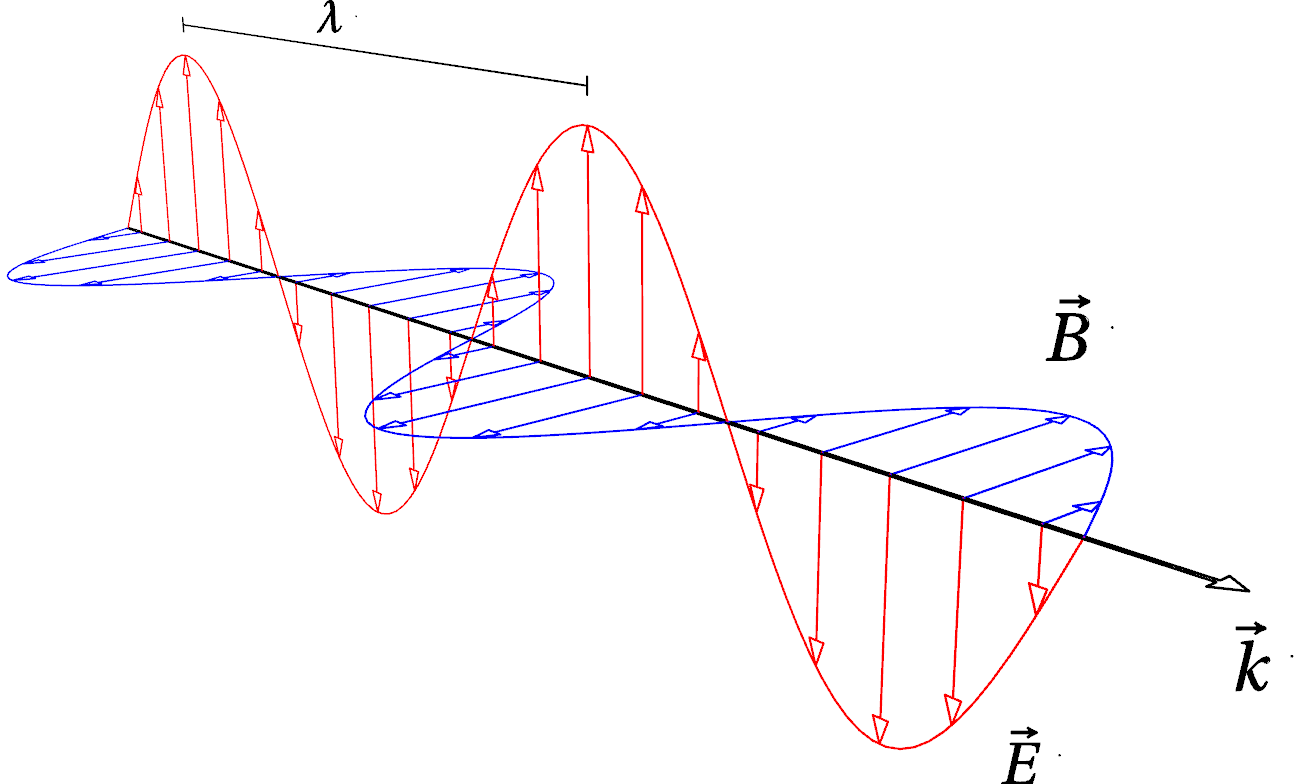
Fig. 4 Vizualization of an electromagnetic (plane) wave. Variable electric \(\vec{E}\) and magnetic \(\vec{B}\) fields are orthogonal to each other and to the direction \(\vec{k}\) of propagation. \(\lambda\) is the wavelength.#
Spectroscopy is the measurement and interpretation of electromagnetic spectra, which offers a powerful toolkit to study the interactions between matter and electromagnetic waves. Historically, spectroscopy begain with studies of electromagnetic radiation in the form of visible light—one could say that our eyes were the first (coarse) spectrometers used for science. However, technological capabilities have gradually developed to cover the whole electromagnetic spectrum: from short-wavelength/high-energy \(\gamma\)- and X-ray radiation through ultraviolet, visible, and infrared light, and our to micro- and radio waves. In this virtual lab, we are using infrared (IR) light (with wavelengths \(\lambda\): 800~nm–1000\(\mu\)m) to study particular types of molecular motion: vibrations and rotations.
Why might we be interested in vibrational and rotational spectroscopy? These techniques allow us to infer the geometric structure of a molecule from its (infrared) absorption spectrum. HCl (shown in Fig. 2) is a highly polar molecule: its atoms carry partial positive +\(q\) and negative −\(q\) charges. These charges interact with the electric field \(\vec{E}\) of an electromagnetic wave and feel a (time-varying) force. As a result, the molecule starts to spin (about its center of mass) and vibrate—where the inter-atomic distance changes when the charges are pushed in opposite directions by the electric field. Both phenomena take place simultaneously, which explains why we are dealing with a composite rotational-vibrational spectrum. Further, vibrations and rotation are not mechanically independent: A the atoms in rotating molecule experience a centrifugal force that stretches the bond, moves the molecule from the natural equilibrium in its inter-atomic potential, and thus perturbs the vibrations. Conversely, vibrations periodically shrink and stretch the bond, changing the distance between atoms and affecting the time-averaged moment of interia. This in turn pertubs the molecular rotation—just like an ice-skater pulling their arms closer to their body to speed up their spin.
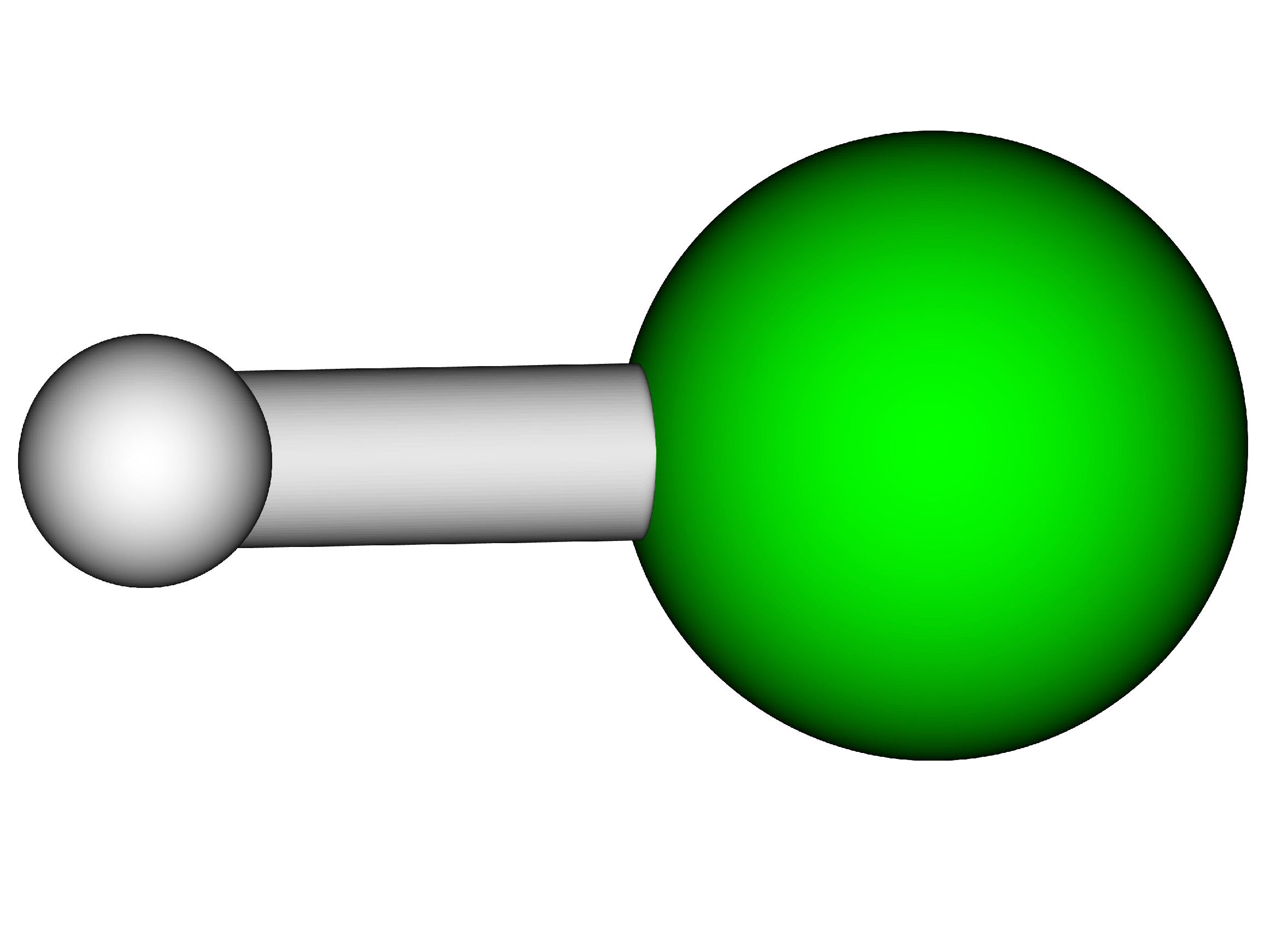
Fig. 5 Structure of the HCl molecule.#
For a diatomic molecule like HCl, we can determine the fundamental vibrational frequency, \(\nu_e\), the rotational constant, \(B_e\), and the vibrational correction term, \(\alpha_e\).* We can then calculate the equilibrium distance \(d_e\) (H–Cl bond length) and the force constant, \(k\), that characterizes the strength of the H–Cl chemical bond.
2 Theory: Vibrations and rotation of a diatomic molecule#
The description of Sec. 1 is based on ideas from the classical chemical structure theory, which assumes the existence of chemical bonds of certain rigidity, partial atomic charges, etc. A more-accurate description of molecular systems, however, is given by the laws of quantum mechanics. Here, we adopt a perturbative treatment, where the (approximate) solutions of the Schrödinger equation provide the rotational-vibrational energy levels \(E_{rv}\) which depend on both the vibrational quantum number \(v = 0, 1, 2, \ldots\) and the rotational quantum number \(J = 0, 1, 2, \ldots\),
(See equations 1 and 2 in the supplementary module on ro-vibrational spectroscopy in the Libretext). Here,
are the equilibrium rotational constant (in SI units) and the harmonic frequency, respectively. Note that \(B=\tilde{B}hc_0\), where \(\tilde{B}\) is the rotational constant expressed in wavenumbers. Other parameters are the equilibrium bond length, \(d_e\), the bond force constant (at the equilibrium position), \(k_e\), and the reduced mass, which for HCl would be:
As follows from Eq. (1), rotational-vibrational energies of a diatomic molecule are quantized: only certain, discrete levels are allowed by quantum mechanics. These levels are not directly observable, though—in spectroscopic experiments we generally infer their energies by looking at transitions between levels. In infrared spectroscopy, we are considering transitions that lead to either the absorption or emission of a photon, and thus our experiments will concern absorption or emission spectra.
2.1 Selection rules#
If all possible transitions between vibrational and rotational energy levels were allowed, a hypothetical spectrum would be quite cluttered in the infrared. However, only a small sub-set of the conceivable trainsitions are usually visible in experimental spectra. These few, allowed transitions are determined by the physical mechanism of interaction between radiation and matter—as was mentioned in Sec. 1, in the general case a diatomic molecule must have a transition dipole (which is the quantum mechanical analog to polar molecules that are classically vibrating or rotating) to exhibit features in an infrared rotational-vibrational spectrum. Quantum mechanically, we can represent this as a matrix element involving the dipole operator, and use the wavefunctions of the quantum harmonic oscillator or rigid rotor to arrive at the selection rules for transitions for a diatomic molecule. In terms of its quantum numbers, these rules imply that the only allowed transitions are those where both quantum numbers change by exactly one:
Allowed transitions are conveniently represented on the energy diagram, Fig. 3.
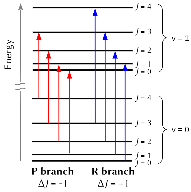
Fig. 6 Energy level diagram and allowed transitions in a rotational-vibrational spectrum of a diatomic molecule. The spacing between vibrational levels (∆v = 1) is large compared to those between rotational ones (∆J = ±1).#
Then, at room temperature, the energy spacing between vibrational levels of HCl is large compared to the characteristic thermal energy, so the overwhelming majority of molecules will be in their ground vibration level prior to exposure to light. As a result the absorption spectrum corresponds to a ∆v = +1 transition (specifically, from \(v=0\), the ground vibrational level to \(v=1\), the first excited state). However, the spacing between the rotational energy levels is comparable to the characteristic thermal energy at room temperature, so a variety of staties (i.e. values of \(J\)) will be initially occupied, and we will observe transitions where the final rotational state is either one greater (\(J_{final}=J_{initial}+1\)), or one less (\(J_{final}=J_{initial}-1\)) than whichever state a particular molecule occupied prior to photoexcitation. Putting this all together, we have a theoretical model for the experimental spectra, which, for HCl, has an appearance siilar to this:
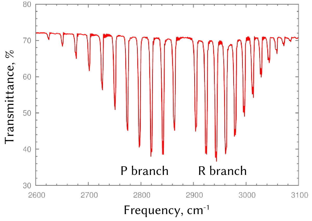
Fig. 7 Rotational-vibrational infrared spectrum of HCl. Note the absence of a Q branch, which would have been located in between P and R branches but is forbidden by selection rules.#
By convention, the series of transitions for which ∆J = −1 is called the P branch, and the series of features for which ∆J = +1 is called the R branch. An R-branch transition originating in state \(J\) and terminating in state \((J + 1)\) is written as \(R(J)\), and a P-branch transition originating in state \(J\) and terminating in state \((J − 1)\) is written as \(P(J)\). Transitions in the Q branch would correspond to a pure vibrational (∆v = 1, ∆J = 0) transition with a frequency \(\nu_e\). Such a transition can be observed in the spectra of more-complex molecules, but it is forbidden to occur (by the previously discussed selection rules) in the rotational-vibrational spectra of simple diatomics, so we will not discuss it further here.
2.2 Structure of the IR spectrum#
An experimental infrared IR spectrum for an HCl molecule is plotted in Fig. 4. It has the expected structure: there are two series of features, the P and R branches, with a gap between them (the missing Q branch). However, we observe that distance between peaks is not quite constant, as the form of Eq. (1) predicted! For example, we could use Eq. (1) to work out the expected photon energies corresponding to transitions for the R branch:
Then, we could consider the distance (in energy) between neighbouring peaks in the spectrum: \(R(J + 1) − R(J) = 2hB_e\). If Eq. (1) were the whole story, the spacing should be a constant!
Thought many possibilities could be considered, it turns out that the dominant reason for this variable spacing is the following: Typically, a molecular vibration is fast—taking place on the order of \(10^{-14} \) s (10 fs!). By comparison, a molecular rotation is usually much slower, taking \(10^{−9}\) s to \(10^{−10}\) s (100 ps - 1 ns). Hence, while a rotating molecule makes one revolution, its atoms undergo many cycles of vibration. This means that the instantaneous bond length will sometimes be longer (and sometimes be shorter) than it is at equilibrium. Because the moment of inertia varies non-linearly with \(d\), this motion has an asymmetric net effect. To account for this, we can replace the \(d_e\) in the definition of the rotational constant, Eq. (2), with a vibrationally averaged \(d\). In the simplest approximation, this leads to a depednence of the rotational constant on \(v\), i.e. the vibrational quantum number. As a result, we end up with a more complicated expression for the (vibrationally-corrected) rotational constant:
Where we have introduced \(\alpha_e\) as a new, empirical constant that captures the strength of this effect for a particular molecule. As a result, the value of the rotational constant now explicitly depends on \(v\). For example, \(B_0\) is the rotational constant for \(v = 0\) and \(B_1\) is the rotational constant when \(v=1\). With this correction, our expression for the rotational-vibrational energy (1) needs to be modified accordingly,
This equation provides the basis for analyzing the vibration-rotation spectrum of HCl.
3 Practical Spectrum Analysis#
Using our new Eq. (7), we can derive expressions for locations of peaks in the R and P branches (where \(\Delta J = +1\) for the former, \(\Delta J = -1\) for the latter, and where \(v_{initial}=0\), \(v_{final}=1\) always, as discussed previously.):
Equations (8) and (9) can be simplified further to assist you in determining \(\nu_e\), \(B_e\), and \(\alpha_e\) directly from the peaks in your experimental spectrum. Specifically, we can introduce a new variable,\(n\) to keep track of sequential features in both branches of the spectrum. We can accomplish this by making the substitution \(n = J_i + 1\) in Eq. (8), and \(n = -J_i\) in Eq. (9), where use \(J_i\) to emphasize that this refers to the rotational state of the molecule before absorption of a photon. This allows us to combine these two expressions together into a single equation for the photon energies at which transitions are expected:
We can now plot the results for both branches of the spectrum on the same graph. Fitting data to a non-linear regression (of a particular functional form you might recognize) by Eq. (10) will yield us several quantities that allow us to calculate our desired physical characteristics of the molecule and allowed transitions.
As a note about units, if our experimental data are plotted versus wavenumbers (i.e. \(\tilde{\nu}_{R,P}(n)\), as is common, it is important to recognize that these values have a linear relation to photon energies given in the expression above. As a result, we can generate the equivalent expression for the key characteristic parameters, \(\tilde{\nu}_e\) , \(\tilde{B}_e\), and \(\alpha_e\) expressed in wavenumbers directly. We thus obtain
For completeness, we emphasize that:
Note that \(c_0=3\times10^{10}\) cm/s must be employed if these expressions are used as-is for dimensional consistancy.